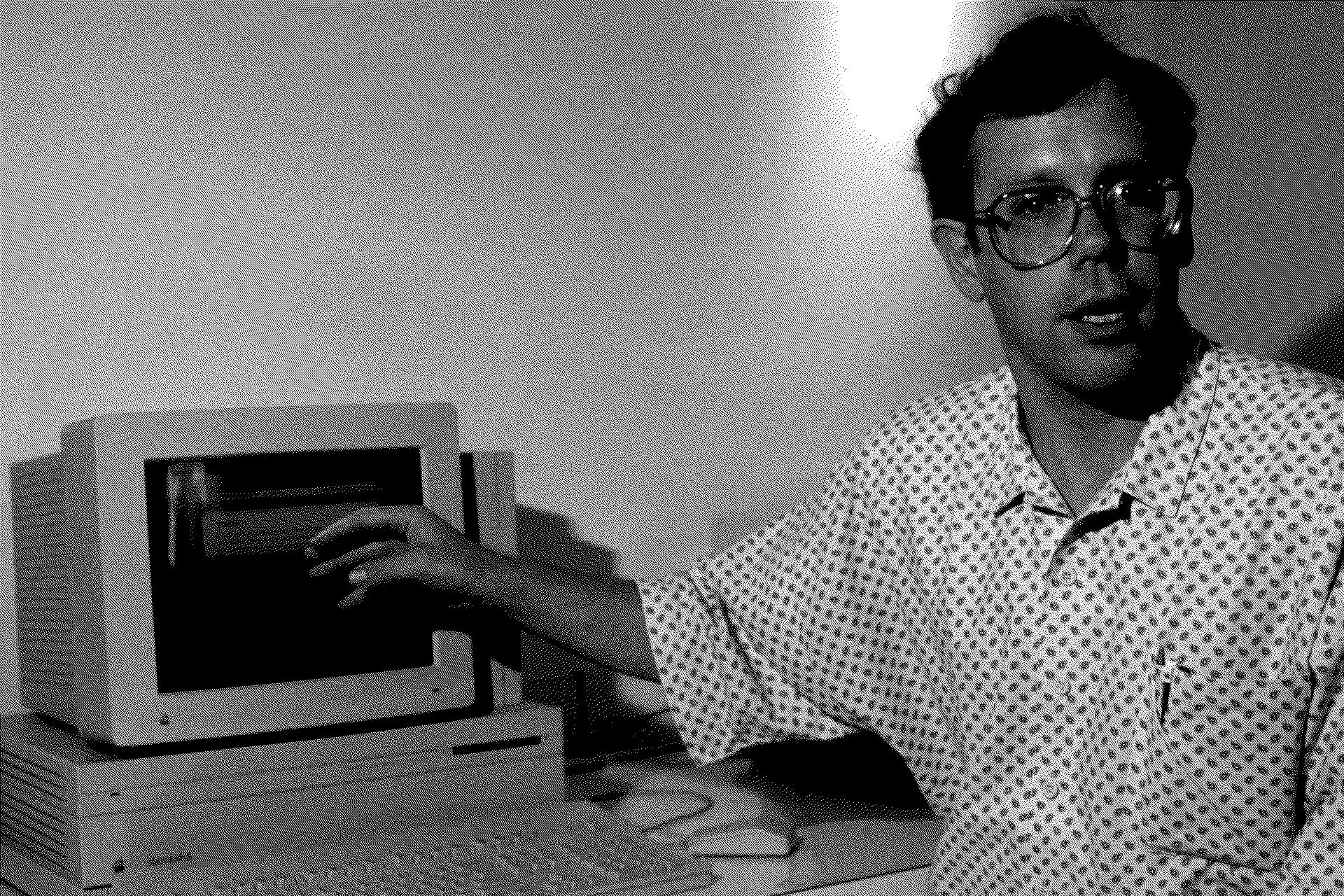
Bill Atkinson and Dithering Algorithms
Simple algorithms are one of my favorite things. They’re quick to learn, elegant, and fun to play with. But importantly, simple algorithms are often the simple solution to a simple problem. Nothing exemplifies this idea more than the Atkinson Dithering algorithm. It is neither the first or best dithering algorithm, but it was a perfect solution for the problem right in front of it on Apple’s original Macintosh. It’s creator, Bill Atkinson, recently passed1 (I know one year is not recently but I am slow at writing so forgive me). I think it’s only fair to honor him with a quick look at one simple algorithm.
Dithering
Dithering a signal is to intentionally add noise in some form or fashion that results in randomizing the quaternization error. Quaternization is when you take something with many inputs, such as 256 colors, and reduce it down to a smaller set of outputs, like 16 colors.
Much like it’s literary definition:
To act nervously or indecisively2
Dithering a signal allows for one to take a function that maps inputs to outputs and make it act a little more nervous in the way it processing pixels to present a more normal looking operation. When dithering images, a by-product of dithering is adding depth to colors.
Dithering algorithms became important in early computer graphics because of limitations of the time. Computer screens could only have so many colors on screen at a time (like black and white or 8 bits of color). Therefore, it became very important to not just be able to display images with the limited color sets but also keep their depth and color. In a few years, this same problem came up on the early internet where images needed to conform to a limited color palette and keep their depth.
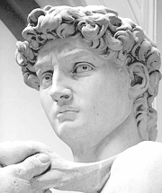
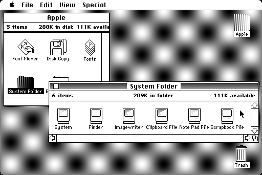
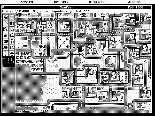
One famous example of this is the GIF standard that limits color palettes to 256 colors. Without dithering, quaternization of reducing an image to 256 colors produces the artifact of color banding. It’s ugly, noticeable, and very easy to fix with dithering.
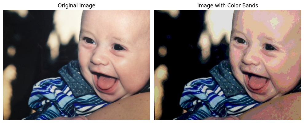
A sampling of algorithms
Floyd-Steinberg
There are many methods to perform dithering for various applications. One can do simple thresholding for a basic solution. Halftoning could be done as well for supporting dot printer operations. A real-time application could reach for a ordered approach that uses a fixed threshold matrix for rendering (like the Return to Obra Dinn3). For our purposes, we will focus on the branch of dithering explored by Bill Atkinson with the original Macintosh: error-diffusion.
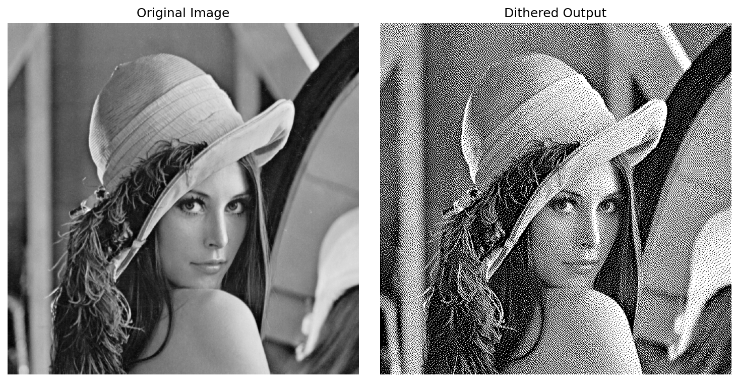
Error-diffusion dithering focuses on dithering by “pushing” the error of the quantization process to neighboring pixels and processing the area of pixels versus a singular pixel at a time. It allows for sharper borders and generally cleaner images on early monitors.
I just want to explore two algorithms and leave the others for readers to explore (maybe even create your own!). The first is Floyd-Steinberg (FS) dithering. The FS algorithm was proposed way back in 1976 by Robert W. Floyd and Louis Steinberg. In case, you were wondering when I brought up the GIF standard earlier, this is the dithering algorithm used in the GIF standard. It is simple and efficient. The best way to understand the process of it to me is to work through the code step by step:
# This code is for black and white images for simplicity
import numpy as np
from PIL import Image

def find_closest_palette_color(pixel: np.float64) -> np.float64:
    if(pixel < 128):
        return 0
    else:
        return 255

def Floyd_Steinberg_Dithering(src_image: np.array) -> np.array:
    # create an output image
    dst_image = np.copy(src_image).astype(np.float64)
    # Find the bounds of the input
    height, width = src_image.shape[:2]

    # Perform dithering operation in raster order (by row then column)
    for row in range(height):
        for col in range(width):
            old_pixel = dst_image[row, col]
            # Find closest match the old pixel color
            new_pixel = find_closest_palette_color(old_pixel)
            # Set output to closest match new pixel
            dst_image[row, col] = new_pixel
            # Find the error from old to new pixel color
            quant_error = old_pixel - new_pixel

            # Diffuse the error to neighboring pixels
            if col + 1 < width:
                dst_image[row, col + 1] += quant_error * 7/16
            if col - 1 >= 0 and row + 1 < height:
                dst_image[row + 1, col - 1] += quant_error * 3/16
            if row + 1 < height:
                dst_image[row + 1, col] += quant_error * 5/16
            if col + 1 < width and row + 1 < height:
                dst_image[row + 1, col + 1] += quant_error * 1/16

    return dst_image
Dithering starts by creating an output image of the same size and shape. The process is about taking something visually complex and making it simpler for later processing and displaying. It is important to keep track of bounds and other parameters that should change.
The process of dithering is performed in raster order. Or in simpler terms, from pixel 0 in the image sequentially left to right to the last pixel. One of the weirdest things to me when I started looking into dithering was understanding raster order (especially with Pillow’s reverse row-column (y,x) accessing). When the quantization error is diffused, it is diffused into the future of the raster order. That means the error only ever diffuses to the right (increasing column number) or down (increasing row number). Every error-diffused dithering algorithm is processed this way. Moreover, processing sequentially is one of the main reason dithering is performed on the CPU and not the GPU.
The algorithm starting at pixel 0. To find what the pixel will be, the algorithm finds the closest color on whatever palette it is given. In this example, it is either black or white. If the image is given in color, the programmer must take that into account.
After finding the closest related color, the actual quantization error is found. It is simply the Euclidean distance from the old color to the new color. But here comes the diffusion part of the error-diffusion. That error value is then divided into slices of a pie and added to it’s neighboring pixels. An example is provided below.
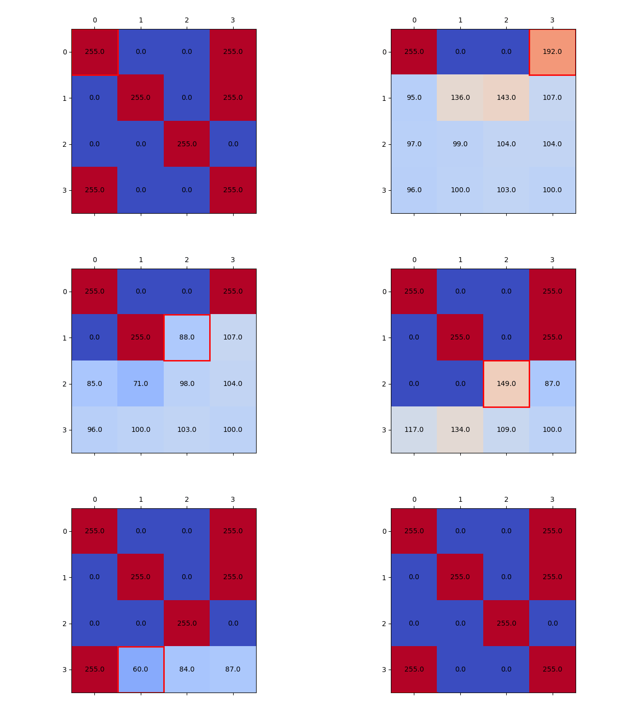
There are two ramification of this process. The first is that the new output pixel will affect what the next output pixel will be. The second is that the diffusion matrix is wildly important in shaping the output. For the FS dithering algorithm the diffusion matrix is (with * denote the current pixel):
\[\begin{bmatrix} & * & \frac{7}{16} \\ \frac{3}{16} & \frac{5}{16} & \frac{1}{16} \end{bmatrix}\]But other algorithms will play with this diffusion matrix to fine-tune their approaches.
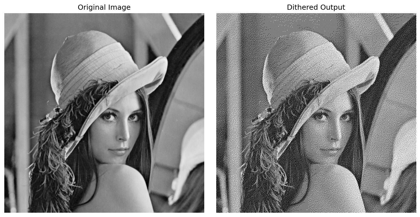
Every pixel is then process in this same way sequentially until the last pixel is reached. Now you’ve taken an image of 256 colors and made it an image of 2 colors in the matter of milliseconds.
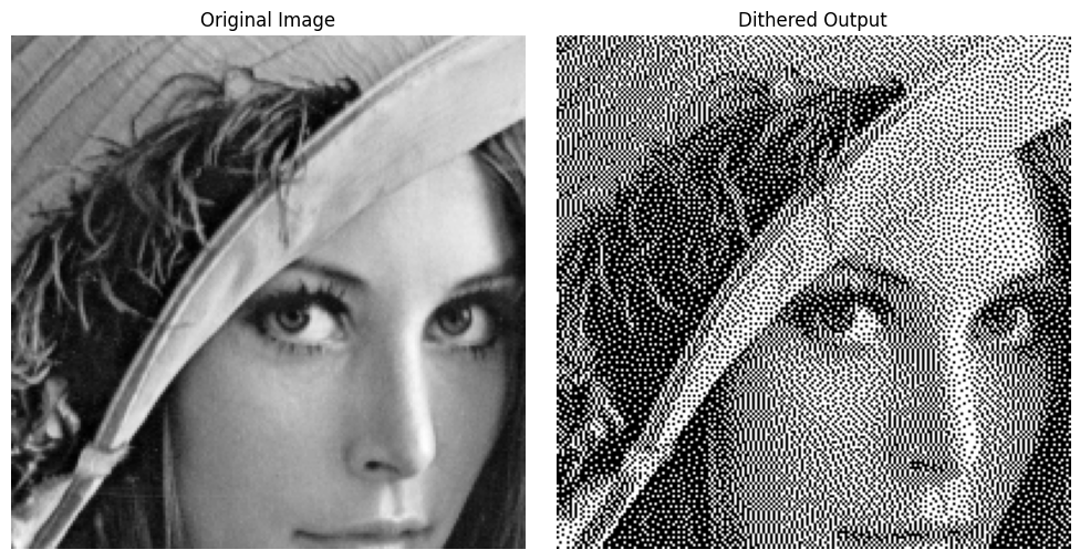
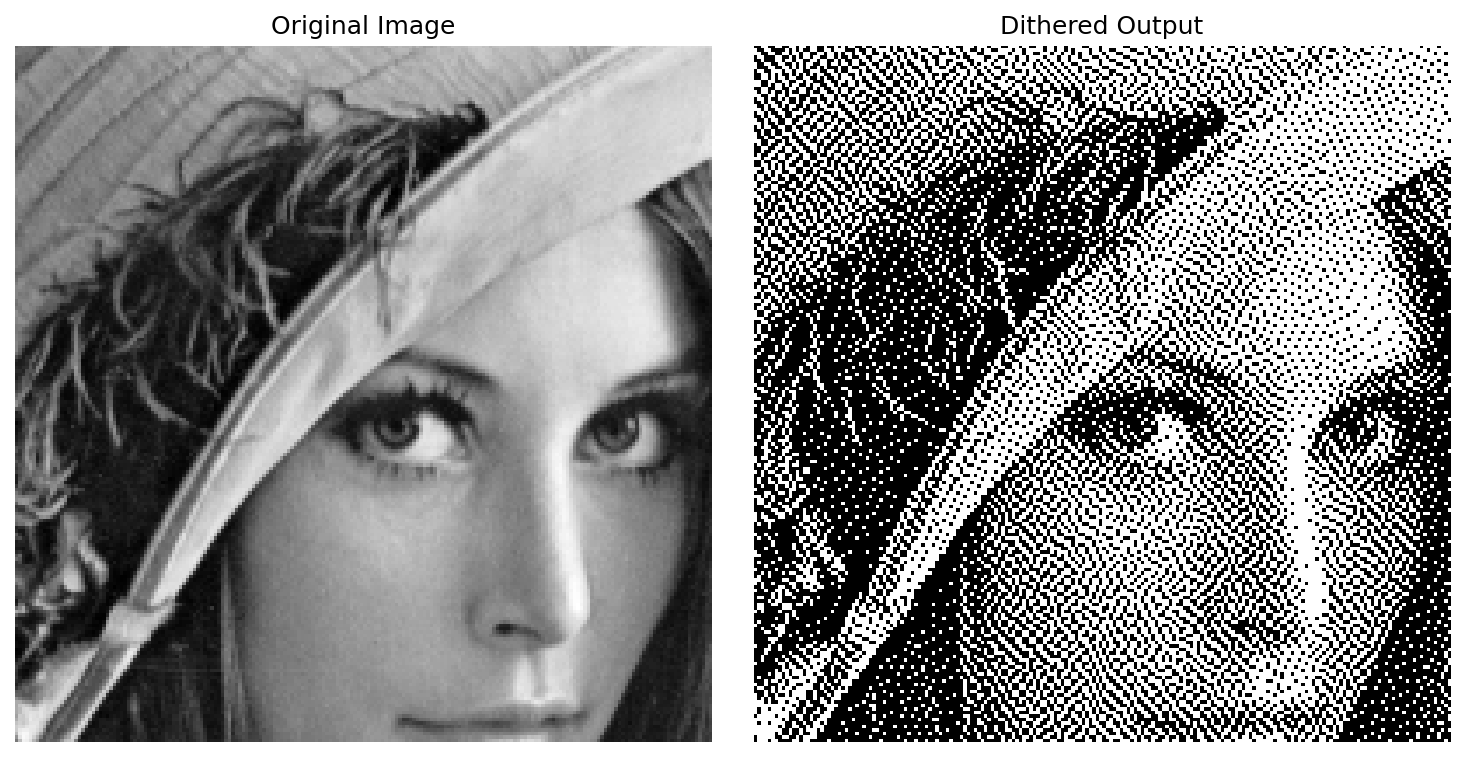
To see the dithering effect alittle more clearly, here is the image zoomed in to the center.
Atkinson
The Macintosh was released in the mythical year of 1984 with a 512x342 pixel screen. The Mac paved the way for modern computers as we know them. It was all-in-one. A mouse and keyboard allow users to interact with both the command-line and a new graphical interface. But the only problem was that the graphical interface was only a CRT monochrome (one color with 0 to 255 values) display. And an engineer at Apple Computer named Bill Atkinson had to make everything look good on this display, no matter what it was.
Atkinson built off the Floyd-Steinberg dithering algorithm with a few modification. The first was that the error would be spread over a larger area rather than just immediate neighbors, like in FS. The second was that only 3/4 of the error would be diffused. The resulting diffusion matrix is below:
\[\begin{bmatrix} & * & \frac{1}{8} & \frac{1}{8} \\ \frac{1}{8} & \frac{1}{8} & \frac{1}{8} \\ & \frac{1}{8} & & \end{bmatrix}\]The result of these two modification was objectively better looking dithering to the human eye. Since only 75% of the quantization error is diffused in the process in a larger area, the effect of the dithering is more localized. Another side effect being that areas of mostly black and white are preserved (so that effects over detail are emphasized4).
The difference of the error diffusion step really emphasizes Atkinson’s changes.
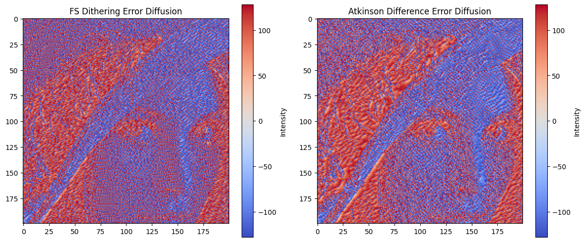
The implementation barely changes as well except for accounting for bounds two rows and columns away.
def Atkinson_Dithering(src_image: np.array) -> np.array:
    dst_image = np.copy(src_image).astype(np.float64)
    height, width = src_image.shape[:2]

    # Same pixel iteration as before
    for row in range(height):
        for col in range(width):
            old_pixel = dst_image[row, col]
            new_pixel = find_closest_palette_color(old_pixel)
            dst_image[row, col] = new_pixel
            quant_error = old_pixel - new_pixel

            # 3/4 Error Diffusion with expanded bounds
            if x + 1 < width:
                dst_image[row, col + 1] += quant_error * 1/8
            if x + 2 < width:
                dst_image[row, col + 2] += quant_error * 1/8
            if row + 1 < height:
                if x - 1 >= 0:
                    dst_image[row + 1, col - 1] += quant_error * 1/8
                dst_image[row + 1, col] += quant_error * 1/8
                if col + 1 < width:
                    dst_image[row + 1, col + 1] += quant_error * 1/8
            if row + 2 < height:
                dst_image[row + 2, col] += quant_error * 1/8

    return dst_image
Some others
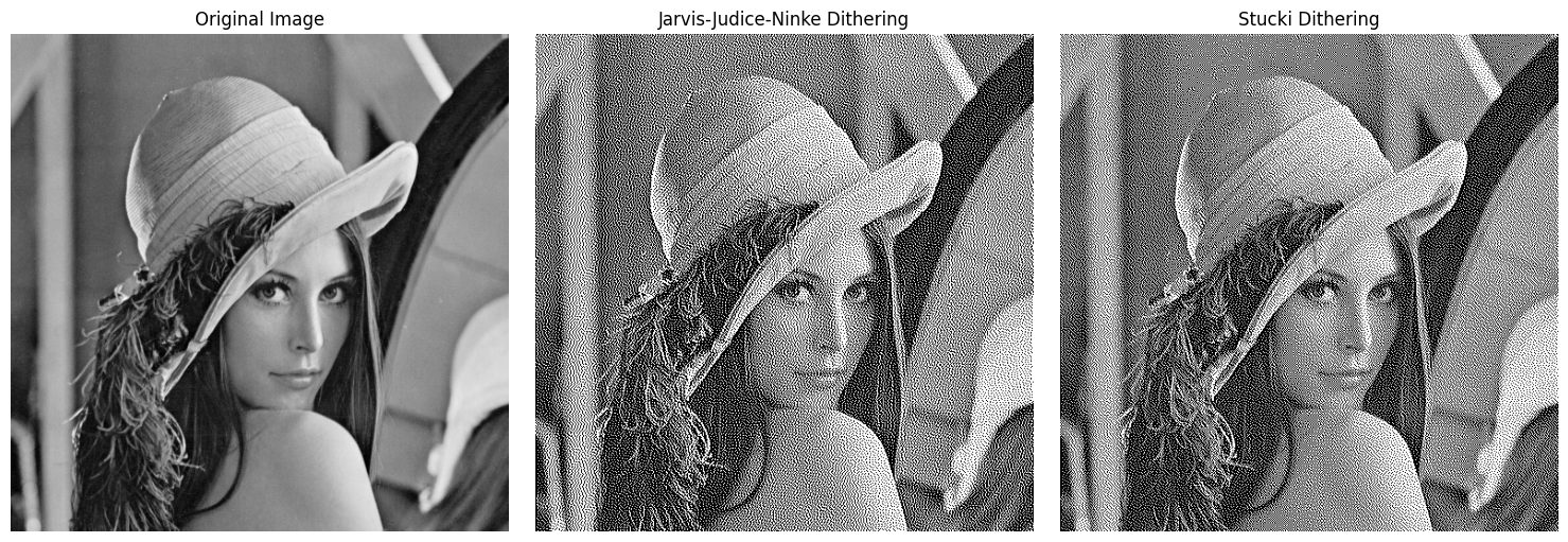
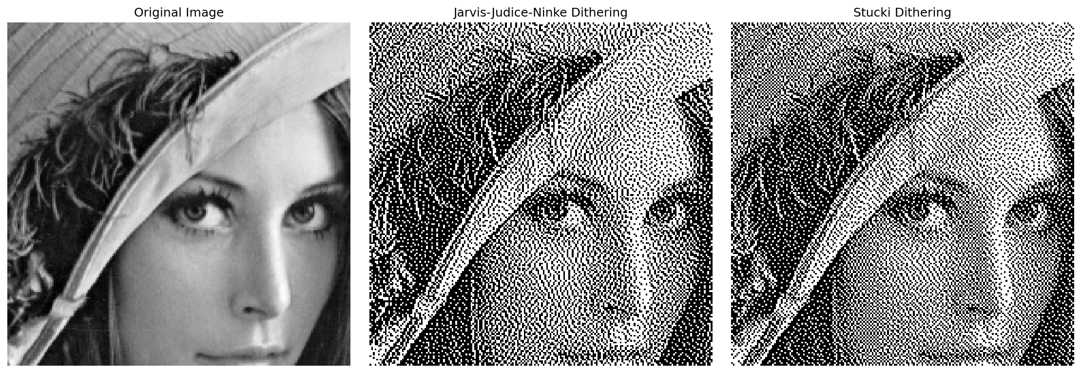
Other variations exist with dithering for different purposes. Minimize Average Error Dithering from Jarvis, Judice, and Ninke (dibs on that 70’s prog band name) distributes the quaternization error even further than the Atkinson algorithm to preserve more details but at the cost of more computation time. Stucki dithering improved on JJN dithering’s computational time by making the kernel all divisible by 2. And so many more! Explore with creating your own kernels5 and become apart of the Ditherpunk movement6.
Simple Algorithms are best
I hope you came away with an appreciation for the simple. Dithering is just one example of something that I think computing has lost in this current age. We want complexity. We want to rush to new technologies because they solve hard things. I myself am guilty of this mindset. I’ll spend days vibe-coding away on problems with hundreds of tokens. But I found, in the end, all it needed was a simple algorithm that took 5 minutes to implement because of the work of a great engineer before me. RIP Bill Atkinson.
Sources
Code for the project can be found at this repo if you want to explore further.